Comparing linear and Additive logistic regression

generalized additive models

generalized linear models

logistic regression

purchasing behaviour

Published

11 February 2024

Library setup

library(mgcv)
library(tidyverse)
library(tidymodels)
library(rstatix)
library(kableExtra)
library(flextable)
library(ggthemes)

Read in the data

Table 1: the first six rows in our data
X	n_acts	bal_crdt_ratio	avg_prem_balance	retail_crdt_ratio	avg_fin_balance	mortgage_age	cred_limit
1	11	0.000	2494.414	0.000	1767.197	182.00	12500
2	0	36.095	2494.414	11.491	1767.197	138.96	0
3	6	17.600	2494.414	0.000	0.000	138.96	0
4	8	12.500	2494.414	0.800	1021.000	138.96	0
5	8	59.100	2494.414	20.800	797.000	93.00	0
6	1	90.100	2494.414	11.491	4953.000	138.96	0

clean up the data

csale_clean<-csale |> 
  select(-X) |> 
  mutate(purchase=as.factor(purchase))

colSums(is.na(csale_clean))
#>          purchase            n_acts    bal_crdt_ratio  avg_prem_balance 
#>                 0                 0                 0                 0 
#> retail_crdt_ratio   avg_fin_balance      mortgage_age        cred_limit 
#>                 0                 0                 0                 0

look at the distribution of the data

csale_clean |> 
  select_if(is.numeric) |> 
  gather() |> 
  ggplot(aes(value)) + 
  geom_density(adjust = 3, col = "#CC9933", fill = "firebrick", alpha = 0.5) +
  facet_wrap(~key,scales="free")+
  theme(axis.text.x = element_text(angle = 60))+
  theme_tufte()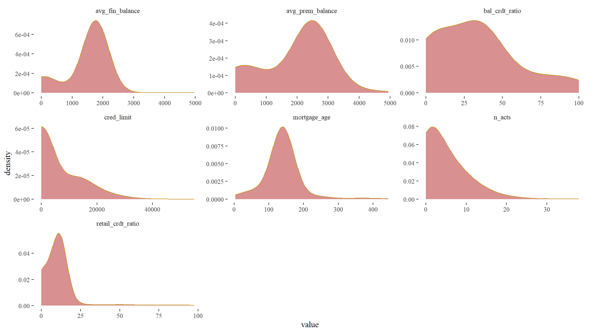

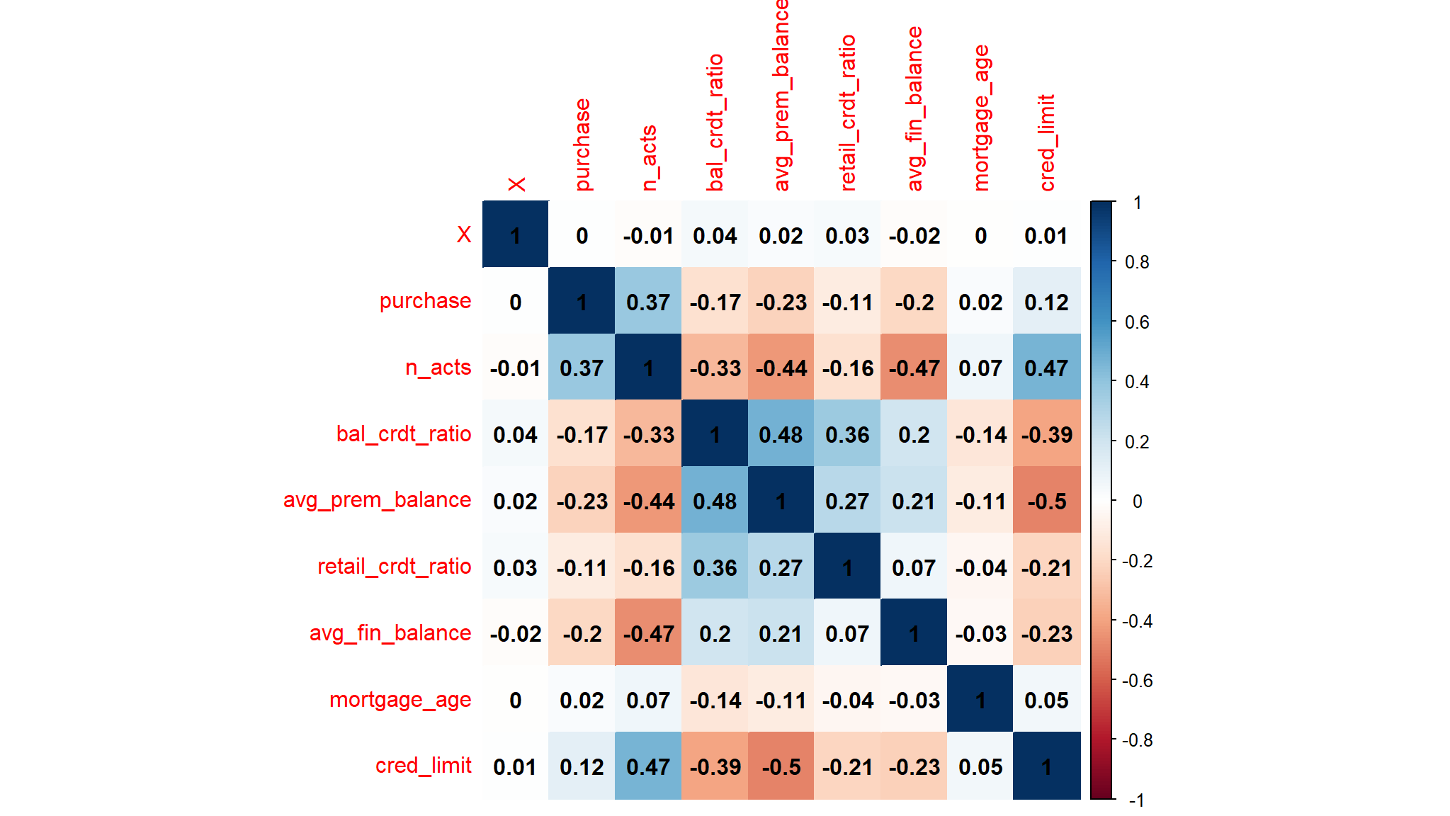
correlation

Initial model development

GLM logistic

# Fit a logistic model
log_mod_glm <- glm(purchase ~ mortgage_age, data = csale,
               family = binomial)
summary(log_mod_glm)
#> 
#> Call:
#> glm(formula = purchase ~ mortgage_age, family = binomial, data = csale)
#> 
#> Coefficients:
#>              Estimate Std. Error z value Pr(>|z|)    
#> (Intercept)  -1.46292    0.16659  -8.781   <2e-16 ***
#> mortgage_age  0.00103    0.00112   0.919    0.358    
#> ---
#> Signif. codes:  0 '***' 0.001 '**' 0.01 '*' 0.05 '.' 0.1 ' ' 1
#> 
#> (Dispersion parameter for binomial family taken to be 1)
#> 
#>     Null deviance: 1832.4  on 1778  degrees of freedom
#> Residual deviance: 1831.6  on 1777  degrees of freedom
#> AIC: 1835.6
#> 
#> Number of Fisher Scoring iterations: 4

AIC(log_mod_glm)
#> [1] 1835.554

GAM logistic

# Fit a logistic model
log_mod_gam <- gam(purchase ~ s(mortgage_age), data = csale,
               family = binomial,
               method = "REML")
summary(log_mod_gam)
#> 
#> Family: binomial 
#> Link function: logit 
#> 
#> Formula:
#> purchase ~ s(mortgage_age)
#> 
#> Parametric coefficients:
#>             Estimate Std. Error z value Pr(>|z|)    
#> (Intercept) -1.34131    0.05908   -22.7   <2e-16 ***
#> ---
#> Signif. codes:  0 '***' 0.001 '**' 0.01 '*' 0.05 '.' 0.1 ' ' 1
#> 
#> Approximate significance of smooth terms:
#>                   edf Ref.df Chi.sq  p-value    
#> s(mortgage_age) 5.226  6.317  30.02 4.11e-05 ***
#> ---
#> Signif. codes:  0 '***' 0.001 '**' 0.01 '*' 0.05 '.' 0.1 ' ' 1
#> 
#> R-sq.(adj) =  0.0182   Deviance explained =  1.9%
#> -REML = 910.49  Scale est. = 1         n = 1779

AIC(log_mod_gam)
#> [1] 1811.976

anova(log_mod_glm,log_mod_gam,test="LRT")
#> Analysis of Deviance Table
#> 
#> Model 1: purchase ~ mortgage_age
#> Model 2: purchase ~ s(mortgage_age)
#>   Resid. Df Resid. Dev     Df Deviance  Pr(>Chi)    
#> 1    1777.0     1831.5                              
#> 2    1772.8     1797.6 4.2261   33.963 9.982e-07 ***
#> ---
#> Signif. codes:  0 '***' 0.001 '**' 0.01 '*' 0.05 '.' 0.1 ' ' 1

Comment

the AIC already suggests that a logistic model under a GAM is better than that in a GLM
The anova test also suggests that a model with a smooth term performs better than the one without

# Calculate the probability at the mean
plogis(coef(log_mod_gam)[1])
#> (Intercept) 
#>    0.207295
plogis(coef(log_mod_glm)[1])
#> (Intercept) 
#>   0.1880214

fit a full model

GAM logistic

# Fit a logistic model
log_mod_gam2 <- gam(purchase ~ s(n_acts) + s(bal_crdt_ratio) +
                  s(avg_prem_balance) + s(retail_crdt_ratio) +
                  s(avg_fin_balance)  + s(mortgage_age) +
                  s(cred_limit),
                data = csale,
                family = binomial,
                method = "REML")

# View the summary
summary(log_mod_gam2)
#> 
#> Family: binomial 
#> Link function: logit 
#> 
#> Formula:
#> purchase ~ s(n_acts) + s(bal_crdt_ratio) + s(avg_prem_balance) + 
#>     s(retail_crdt_ratio) + s(avg_fin_balance) + s(mortgage_age) + 
#>     s(cred_limit)
#> 
#> Parametric coefficients:
#>             Estimate Std. Error z value Pr(>|z|)    
#> (Intercept) -1.64060    0.07557  -21.71   <2e-16 ***
#> ---
#> Signif. codes:  0 '***' 0.001 '**' 0.01 '*' 0.05 '.' 0.1 ' ' 1
#> 
#> Approximate significance of smooth terms:
#>                        edf Ref.df Chi.sq  p-value    
#> s(n_acts)            3.474  4.310 93.670  < 2e-16 ***
#> s(bal_crdt_ratio)    4.308  5.257 18.386  0.00319 ** 
#> s(avg_prem_balance)  2.275  2.816  7.800  0.04889 *  
#> s(retail_crdt_ratio) 1.001  1.001  1.422  0.23343    
#> s(avg_fin_balance)   1.850  2.202  2.506  0.27889    
#> s(mortgage_age)      4.669  5.710  9.656  0.13356    
#> s(cred_limit)        1.001  1.002 23.066 2.37e-06 ***
#> ---
#> Signif. codes:  0 '***' 0.001 '**' 0.01 '*' 0.05 '.' 0.1 ' ' 1
#> 
#> R-sq.(adj) =  0.184   Deviance explained = 18.4%
#> -REML = 781.37  Scale est. = 1         n = 1779

AIC(log_mod_gam2)
#> [1] 1542.598


# Plot on the log-odds scale
plot(log_mod_gam2, pages = 1)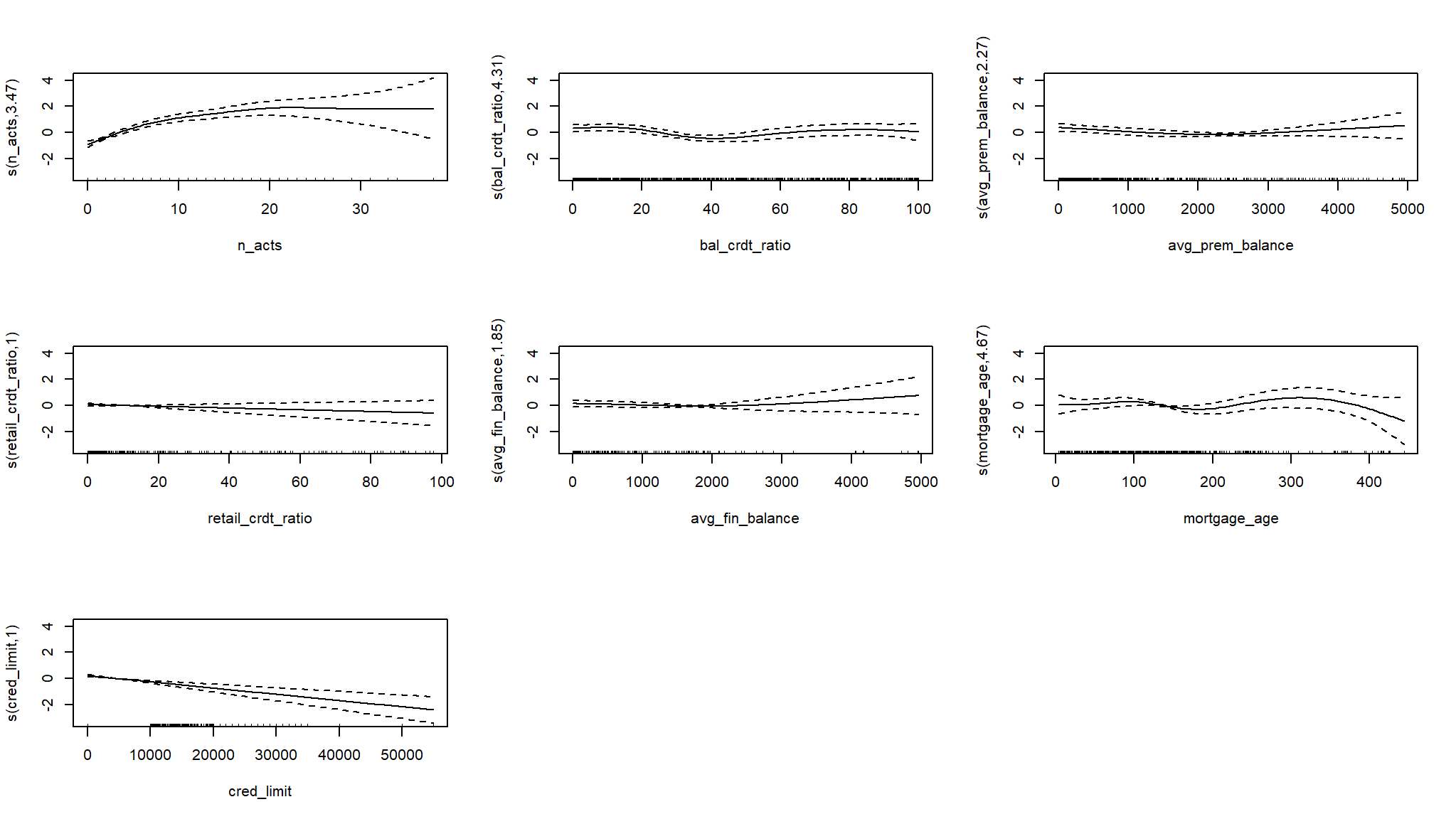


# Plot on the probability scale
plot(log_mod_gam2, pages = 1, trans = plogis)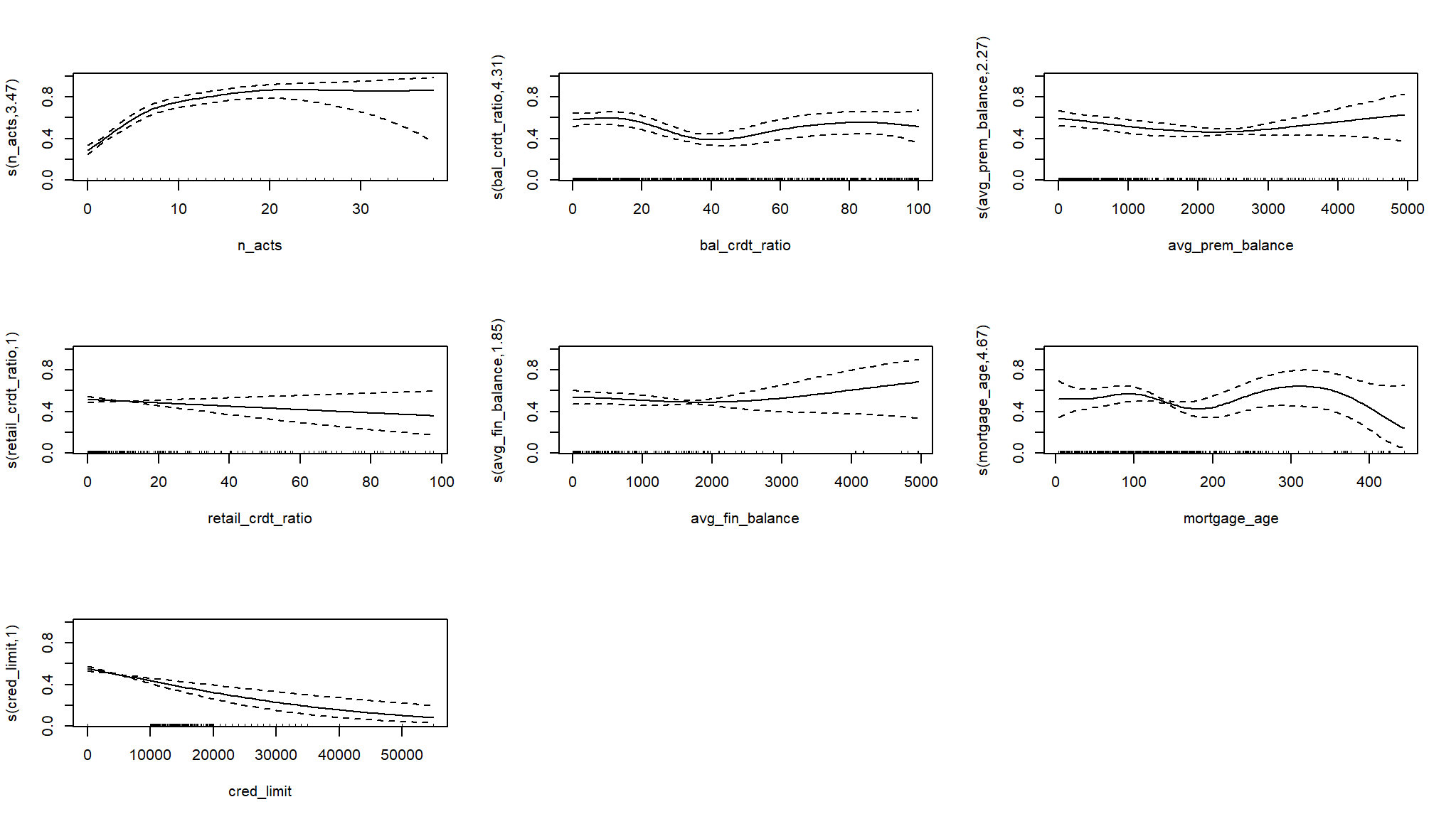


# Plot with the intercept
plot(log_mod_gam2, pages = 1, trans = plogis,
     shift = coef(log_mod_gam2)[1])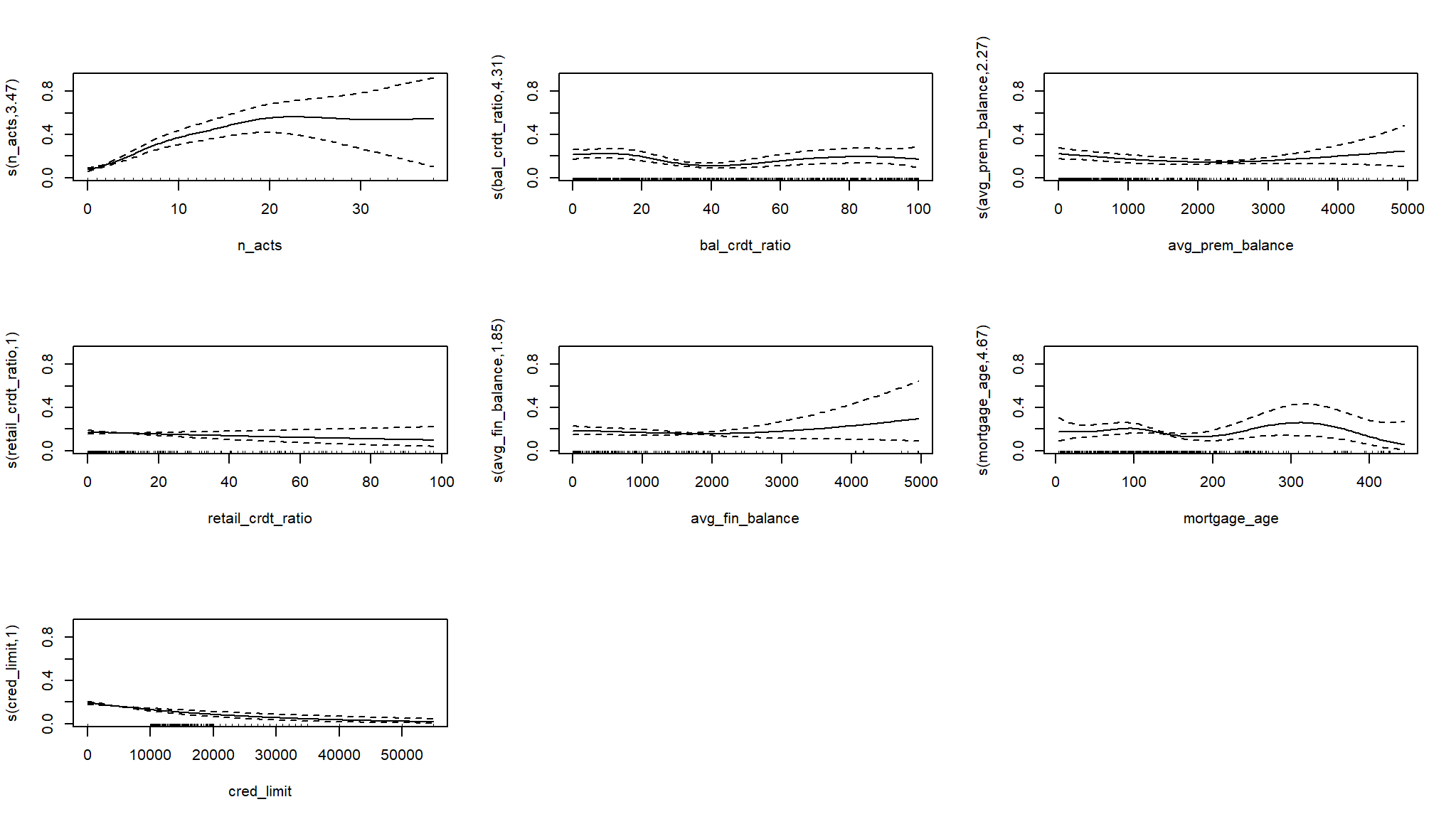


# Plot with intercept uncertainty
plot(log_mod_gam2, pages = 1, trans = plogis,
     shift = coef(log_mod_gam2)[1], seWithMean = TRUE,
     rug = FALSE, shade = TRUE, shade.col = "lightgreen" , col = "purple")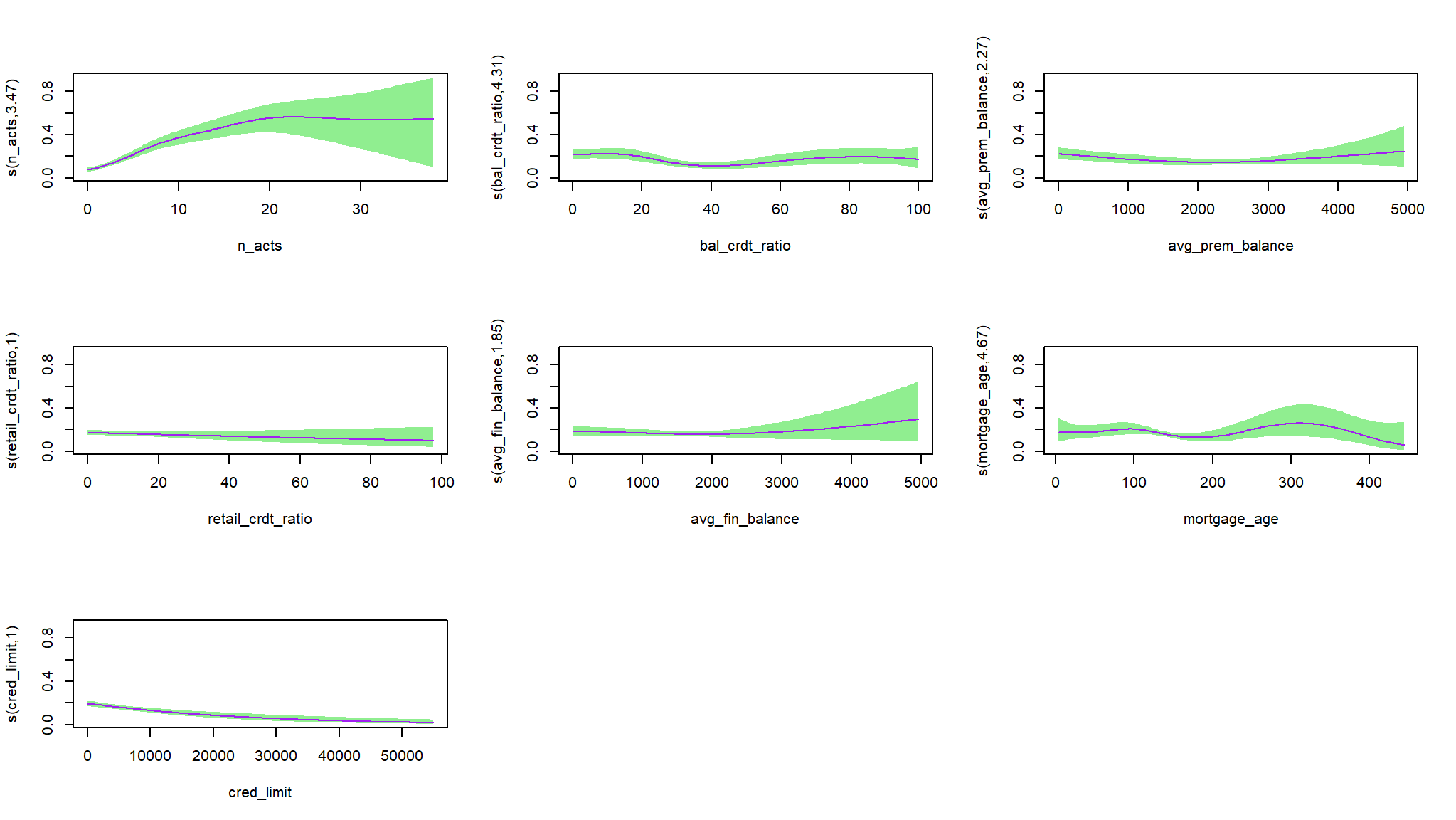

GLM logistic

log_m <- glm(purchase ~ n_acts + bal_crdt_ratio +
                avg_prem_balance + retail_crdt_ratio +
                  avg_fin_balance  + mortgage_age +
                  cred_limit,
                data = csale,
                family = binomial)
summary(log_m)
#> 
#> Call:
#> glm(formula = purchase ~ n_acts + bal_crdt_ratio + avg_prem_balance + 
#>     retail_crdt_ratio + avg_fin_balance + mortgage_age + cred_limit, 
#>     family = binomial, data = csale)
#> 
#> Coefficients:
#>                     Estimate Std. Error z value Pr(>|z|)    
#> (Intercept)       -1.052e+00  2.901e-01  -3.628 0.000285 ***
#> n_acts             1.483e-01  1.467e-02  10.109  < 2e-16 ***
#> bal_crdt_ratio    -4.485e-03  3.003e-03  -1.493 0.135310    
#> avg_prem_balance  -2.335e-04  7.006e-05  -3.333 0.000860 ***
#> retail_crdt_ratio -6.247e-03  5.916e-03  -1.056 0.291052    
#> avg_fin_balance   -1.157e-04  9.104e-05  -1.271 0.203606    
#> mortgage_age      -8.033e-04  1.134e-03  -0.709 0.478596    
#> cred_limit        -3.718e-05  9.579e-06  -3.881 0.000104 ***
#> ---
#> Signif. codes:  0 '***' 0.001 '**' 0.01 '*' 0.05 '.' 0.1 ' ' 1
#> 
#> (Dispersion parameter for binomial family taken to be 1)
#> 
#>     Null deviance: 1832.4  on 1778  degrees of freedom
#> Residual deviance: 1580.0  on 1771  degrees of freedom
#> AIC: 1596
#> 
#> Number of Fisher Scoring iterations: 4

AIC(log_m)
#> [1] 1596.011

comments

again the GAM logistic performs better with a much smaller AIC

Lets see how these compare on new predictions

set up data for modeling

set.seed(123)
csale<-csale |> 
  mutate(purchase=as.factor(purchase)) |> 
  select(-X)

# Split the dataset 
td_split <-initial_split(csale, strata = purchase, prop=0.75)

train <- training(td_split)
test <- testing(td_split)

set up a recipe

train_rcp <- recipe(purchase ~ ., data=csale)

# Prep and bake the recipe so we can view this as a seperate data frame
training_df <- train_rcp |> 
  prep() |> 
  juice()

Set up engines for different models

initialise a GLM model

log_mod_glm <- logistic_reg() |> 
          set_engine('glm') |> 
          set_mode("classification")

add to workflow

lr_wf <-
  workflow() |> 
  add_model(log_mod_glm) |> 
  add_recipe(train_rcp)

lr_fit <- 
  lr_wf |> 
  fit(data=train)

Extracting the fitted data

I want to pull the data fits into a tibble I can explore. This can be done below:

lr_fitted <- lr_fit |> 
  extract_fit_parsnip() |> 
  tidy()

I will visualise this via a bar chart to observe my significant features:

Use fitted logistic regression model to predict on test set

We are going to now append our predictions from our model we created as a baseline to append to the predictions we already have in the predictions data frame:

testing_lr_fit_probs <- predict(lr_fit, test, type='prob')
testing_lr_fit_class <- predict(lr_fit, test)

predictions<- cbind(test, testing_lr_fit_probs, testing_lr_fit_class)

predictions <- predictions |> 
  dplyr::mutate(log_reg_model_pred=.pred_class,
                log_reg_model_prob=.pred_1) |> 
  dplyr::select(everything(), -c(.pred_class, .pred_0)) |> 
  dplyr::mutate(log_reg_class_custom = ifelse(log_reg_model_prob >0.7,"Yes","No")) |> 
  dplyr::select(-.pred_1)

Confusion matrix

predictions |> 
  conf_mat(purchase,log_reg_model_pred)
#>           Truth
#> Prediction   0   1
#>          0 340  72
#>          1  11  22

predictions |> 
  conf_mat(purchase,log_reg_model_pred) |> 
  autoplot(type="heatmap")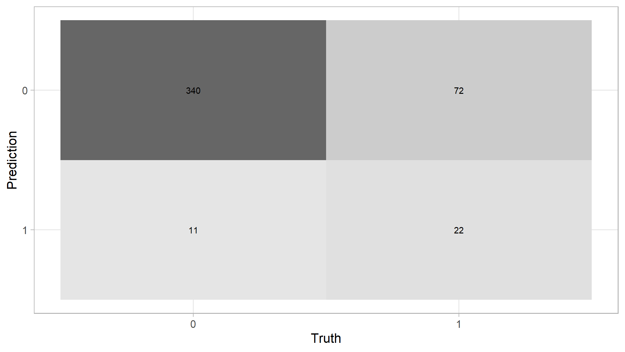

.metric	.estimator	.estimate
ppv	binary	0.8252427
recall	binary	0.9686610
accuracy	binary	0.8134831
f_meas	binary	0.8912189

initialise a GAM model

log_mod_gam <- gen_additive_mod() |> 
  set_engine('mgcv',method="REML") |> 
  set_mode("classification")

add to workflow

lr_fit <-log_mod_gam |> 
  fit(purchase ~ s(n_acts) + s(bal_crdt_ratio) +
                  s(avg_prem_balance) + s(retail_crdt_ratio) +
                  s(avg_fin_balance)  + s(mortgage_age) +
                  s(cred_limit),data=train)

Extracting the fitted data

I want to pull the data fits into a tibble I can explore. This can be done below:

lr_fitted <- lr_fit |> 
  tidy()

I will visualise this via a bar chart to observe my significant features:

Use fitted logistic regression model to predict on test set

We are going to now append our predictions from our model we created as a baseline to append to the predictions we already have in the predictions data frame:

predictions |> 
  conf_mat(purchase,log_reg_model_pred)
#>           Truth
#> Prediction   0   1
#>          0 335  72
#>          1  16  22

predictions |> 
  conf_mat(purchase,log_reg_model_pred) |> 
  autoplot(type="heatmap")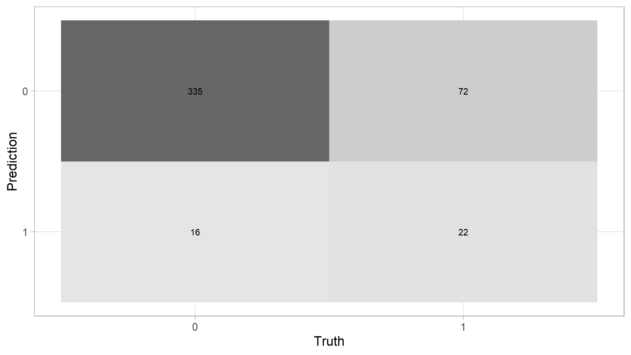

.metric	.estimator	.estimate
ppv	binary	0.8230958
recall	binary	0.9544160
accuracy	binary	0.8022472
f_meas	binary	0.8839050

Note

The generalised Additive logistic regression performs a bit poor than the glm
the difference is just one percent accuracy